HR Metrics Every People Analytics Team Should Track

people analytics

HR metrics

tutorial

A practical introduction to the core KPIs in workforce analytics — with R code to calculate them yourself.

Author

Felix Betancourt

Published

April 1, 2026

Why HR Metrics Matter

Most HR departments collect data. Far fewer actually use it. The gap between having a spreadsheet and having insight is where People Analytics lives.

In this post I’ll walk through the five foundational HR metrics every analytics-capable team should have on their dashboard — and show how to calculate them in R.

Setup

Code

library(tidyverse)

# Simulated employee dataset
set.seed(42)
n <- 500

employees <- tibble(
  employee_id   = 1:n,
  hire_date     = sample(seq(as.Date("2018-01-01"), as.Date("2025-01-01"), by="day"), n, replace=TRUE),
  term_date = sample(c(as.Date(NA), sample(seq(as.Date("2020-01-01"), as.Date("2025-12-31"), by="day"), n, replace=TRUE)), n, replace=TRUE),
  department    = sample(c("Sales","Engineering","HR","Finance","Operations"), n, replace=TRUE),
  salary        = round(rnorm(n, mean=75000, sd=20000)),
  performance   = sample(1:5, n, replace=TRUE, prob=c(0.05,0.15,0.40,0.30,0.10)),
  active        = is.na(term_date)
)

1. Headcount

Code

headcount <- employees |>
  filter(active) |>
  count(department, name = "headcount") |>
  arrange(desc(headcount))

headcount

# A tibble: 2 × 2
  department headcount
  <chr>          <int>
1 Finance            1
2 HR                 1

2. Turnover Rate

Annualized voluntary turnover is one of the most watched metrics in HR:

\[\text{Turnover Rate} = \frac{\text{Separations in Period}}{\text{Average Headcount}} \times 100\]

Code

separations_2024 <- employees |>
  filter(!is.na(term_date), 
         between(term_date, as.Date("2024-01-01"), as.Date("2024-12-31"))) |>
  nrow()

avg_headcount <- employees |>
  filter(hire_date <= as.Date("2024-12-31")) |>
  nrow()

turnover_rate <- (separations_2024 / avg_headcount) * 100

cat("Annual Turnover Rate (2024):", round(turnover_rate, 1), "%")

Annual Turnover Rate (2024): 17.6 %

3. Average Tenure

Code

employees |>
  mutate(
    end_date  = if_else(active, Sys.Date(), term_date),
    tenure_yrs = as.numeric(end_date - hire_date) / 365.25
  ) |>
  group_by(department) |>
  summarise(avg_tenure_years = round(mean(tenure_yrs), 1)) |>
  arrange(desc(avg_tenure_years))

# A tibble: 5 × 2
  department  avg_tenure_years
  <chr>                  <dbl>
1 Finance                  1.5
2 Engineering              1.4
3 HR                       1.4
4 Sales                    1.4
5 Operations               1.1

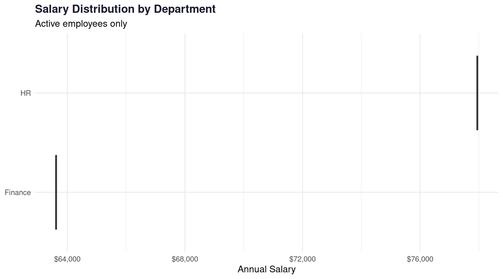
4. Salary Distribution by Department

Code

employees |>
  filter(active) |>
  ggplot(aes(x = reorder(department, salary, median), y = salary, fill = department)) +
  geom_boxplot(alpha = 0.7, show.legend = FALSE) +
  scale_y_continuous(labels = scales::dollar_format()) +
  scale_fill_manual(values = c("#29abe2","#1a7db5","#74c8ec","#0d5c8a","#a8d8ea")) +
  coord_flip() +
  labs(
    title    = "Salary Distribution by Department",
    subtitle = "Active employees only",
    x        = NULL,
    y        = "Annual Salary"
  ) +
  theme_minimal(base_size = 12) +
  theme(plot.title = element_text(color = "#1a1a2e", face = "bold"))

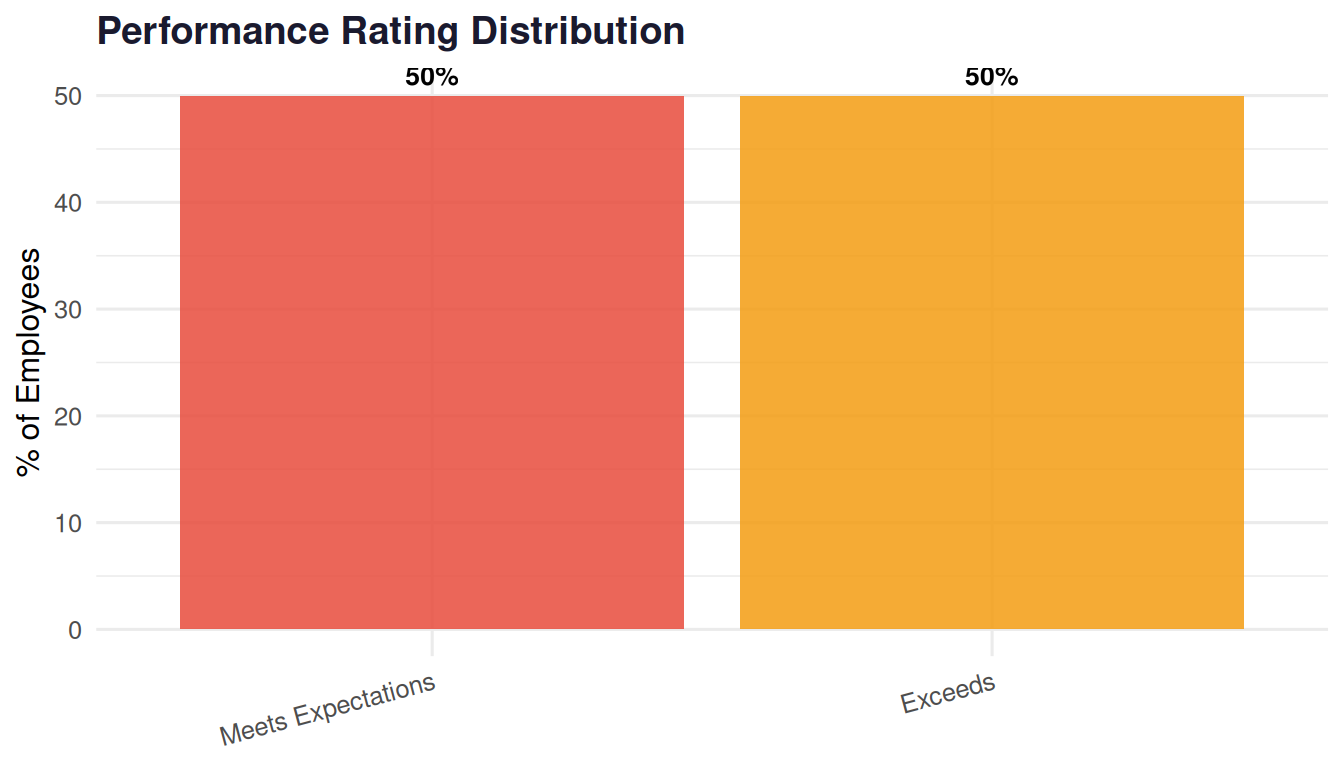
5. Performance Distribution

Code

perf_data <- employees |>
  filter(active) |>
  count(performance) |>
  mutate(
    pct = n / sum(n) * 100,
    label = paste0(round(pct, 1), "%"),
    perf_label = factor(performance, levels = 1:5,
      labels = c("Needs Improvement","Below Average","Meets Expectations","Exceeds","Outstanding"))
  )

ggplot(perf_data, aes(x = perf_label, y = pct, fill = perf_label)) +
  geom_col(show.legend = FALSE, alpha = 0.85) +
  geom_text(aes(label = label), vjust = -0.5, fontface = "bold", size = 3.5) +
  scale_fill_manual(values = c("#e74c3c","#f39c12","#74c8ec","#29abe2","#1a7db5")) +
  labs(title = "Performance Rating Distribution", x = NULL, y = "% of Employees") +
  theme_minimal(base_size = 12) +
  theme(axis.text.x = element_text(angle = 15, hjust = 1),
        plot.title = element_text(color = "#1a1a2e", face = "bold"))

Key Takeaways

These five metrics — headcount, turnover rate, tenure, compensation equity, and performance distribution — are the foundation of any people analytics practice. Once you have these running reliably, you can layer in more advanced work: predictive attrition models, engagement drivers, succession risk.

In upcoming posts I’ll show how to take this further with machine learning and real workforce datasets.

All data in this post is simulated for illustration purposes.

Citation

BibTeX citation:

@online{betancourt2026,
  author = {Betancourt, Felix},
  title = {HR {Metrics} {Every} {People} {Analytics} {Team} {Should}
    {Track}},
  date = {2026-04-01},
  url = {https://www.bluecognition.net/posts/post-with-code/},
  langid = {en}
}

For attribution, please cite this work as:

Betancourt, Felix. 2026. “HR Metrics Every People Analytics Team Should Track.” April 1, 2026. https://www.bluecognition.net/posts/post-with-code/.